4.3 The magic of rio
“The aim of rio is to make data file I/O [import/output] in R as easy as possible by implementing three simple functions in Swiss-army knife style,” according to the project’s GitHub page. Those functions are import(), export(), and convert().
So, the rio package has just one function to read in many different types of files: import(). If you import("myfile.csv"), it knows to use a function to read a CSV file. import("myspreadsheet.xlsx") works the same way. In fact, rio handles more than two dozen formats including tab-separated data (with the extension .tsv), JSON, Stata, and fixed-width format data (.fwf).
Once you’ve analyzed your data, if you want to save the results as a CSV, Excel spreadsheet, or other formats, rio’s export() function can handle that.
You should have installed rio in Chapter 1, but if you skipped that part, install it now with install.packages("rio") .
I’ve set up some sample data with Boston winter snowfall data. You could head to http://bit.ly/BostonSnowfallCSV and right click to save the file as BostonWinterSnowfalls.csv in your current R project working directory. But one of the points of scripting is to replace manual work - tedious or otherwise - with automation that is easy to reproduce. Instead of clicking to download, you can use R’s download.file function with the syntax download.file("url", "destinationFileName.csv"):
This assumes that your system will redirect from that bit.ly URL shortcut and successfully find the real file URL, https://raw.githubusercontent.com/smach/NICAR15data/master/BostonWinterSnowfalls.csv . I’ve occasionally had problems accessing Web content on old Windows machines. If you’ve got one of the those and this bit.ly link isn’t working, you can swap in the actual URL for the bit.ly link. (You may want to use the shortcut link in your browser to get to the longer one that you can copy and paste, instead of typing it out manually. Or, go to http://bit.ly/R4JournalismLinks and copy the link from there). Another option is upgrading your Windows machine to Windows 10 if possible to see if that does the trick.
If you wish that rio could just import data directly from a URL, in fact it can, and I’ll get to that in the next section. The point of this section is to get practice working with a local file.
Once you have the test file on your local system, you can load that data into an R object called snowdata with the code:
Note that it’s possible rio will ask you to re-download the file in binary format, in which case you’ll need to run download.file(“http://bit.ly/BostonSnowfallCSV”, “BostonWinterSnowfalls.csv”, mode=‘wb’).
I want to remind you again about RStudio’s tab completion options if you haven’t been using them. If you type rio:: and wait, you’ll get a list of all available functions. Type snow and wait, and you should see the full name of your object as an option. Use your up and down arrow keys to move between auto-completion suggestions. Once the option you want is highlighted, hit the tab key (or Enter) and the full object or function name will be added to your script.
You should see the object snowdata appear in your environment tab in the RStudio top right pane (if that top right pane is showing your command History instead of your Environment, select the Environment tab). snowdata should show that it has 76 “obs.” – observations, or rows – and 2 variables, or columns. If you click on the arrow to the left of snowdata to expand the listing, you’ll see the 2 column names and the type of data each column holds. The Winter is character strings and the Total column is numeric. You should also be able to see the first few values of each column in the Environment pane.
Click on the word snowdata itself in the Environment tab for a more spreadsheet-like view of your data. You can get that same view from the R console with the command View(snowdata) (that’s got to be a capital V on View - view won’t work). Note: snowdata is not in quotation marks because you are referring to the name of an R object in your environment. In the rio::import command before, “BostonWinterSnowfalls.csv” is in quotation marks because that’s not an R object, it’s a character string name of a file outside of R.
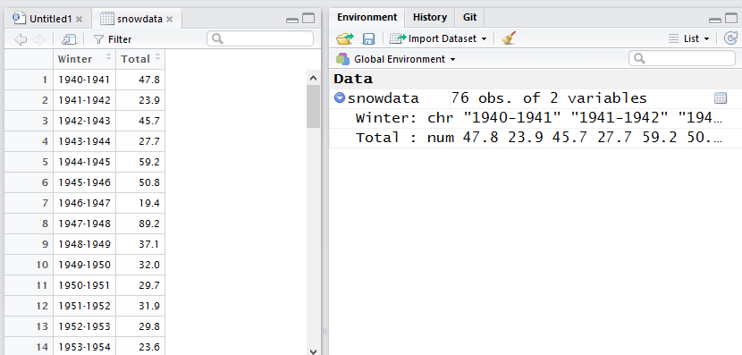
Figure 4.1: Viewing the snowdata R object within RStudio
This view has a couple of spreadsheet-like behaviors, as shown in Figure 4.1. Click on a column header and it will sort by that column’s values in ascending order; click the same column header a second time, and it will sort descending. There’s a search box to find rows matching certain characters.
If you click the Filter icon, you’ll get a filter for each column. The Winter character column works as you might expect, filtering for any rows that contain the characters you type in. If you click in the Total numerical column’s filter, though, older versions of RStudio show a slider while newer ones show a histogram and a box for filtering.
4.3.1 Import a file from the Web
If you want to download and import a file from the Web, you can do so if it’s publicly available and in a format such as Excel or CSV. Try
A lot of systems will be able to follow the redirect URL to the file even after first giving you an error message, as long as you specify the format as “csv” since the file name here doesn’t include “.csv”. If yours won’t, use the URL “https://raw.githubusercontent.com/smach/R4JournalismBook/master/data/BostonSnowfall.csv” instead.
rio can also import well-formatted HTML tables from Web pages, but the tables have to be extremely well-formatted. Let’s say you want to download the table that describes the National Weather Service’s severity ratings for snowstorms. The National Centers for Environmental Information Regional Snowfall Index page has just one table, very well crafted, so code like this should work:
rsi_description <- rio::import("https://www.ncdc.noaa.gov/snow-and-ice/rsi/", format="html")
Note again that you need to include the format, in this case format="html". because the URL itself doesn’t give any indication as to what kind of file it is. If the URL included a file name with an .html extension, rio would know.
In real life, though, Web data rarely appears in such neat, isolated form. A good option for cases that aren’t quite as well crafted is often the htmltab package. Install it with install.packages("htmltab"). The package’s function for reading an HTML table is also called htmltab. But if you run this:
library(htmltab)
citytable <- htmltab("https://en.wikipedia.org/wiki/List_of_United_States_cities_by_population")
str(citytable)
you’ll see that you don’t have the correct table, because the data frame contains one object. Since I didn’t specify which table, it pulled the first HTML table on the page. That didn’t happen to be the one I want. I don’t feel like importing every table on the page until I find the right one, but fortunately, I have a Chrome extension called Table Capture that lets me view a list of all the tables on a page, such as in Figure 4.2.
The last time I checked, table #5 with more than 300 rows was the one I wanted. If that doesn’t work for you now, try installing Table Capture on a Chrome browser to check which table you want to download.
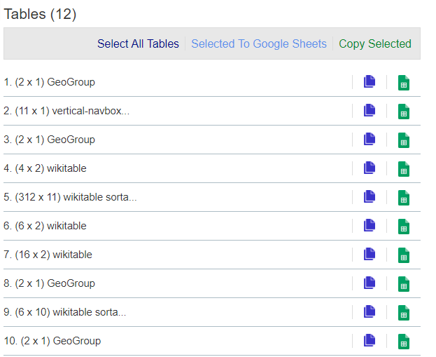
Figure 4.2: The Chrome Table Capture extension.
I’ll try again, specifying table 5 and then seeing what column names are in the new citytable. Note that in the following code, I put the citytable <- htmltab() command onto multiple lines. That’s so it didn’t run off the printed page – you can keep everything on a single line. If the table number has changed since publication, replace which = 5 with the correct number.
Instead of using the page at Wikipedia, you can replace the Wikipedia URL with the URL of a copy of the file I created. That file is at http://bit.ly/WikiCityList. To use that version, type bit.ly/WikiCityList into a browser, then copy the lengthy URL it redirects to and use that instead of the wikipedia.org URL below:
library(htmltab)
citytable <- htmltab(
  "https://en.wikipedia.org/wiki/List_of_United_States_cities_by_population",
  which = 5)
colnames(citytable)
## [1] "2017rank" "City"
## [3] "State" "2017estimate"
## [5] "2010Census" "Change"
## [7] "2016 land area" "2016 land area"
## [9] "2016 population density" "2016 population density"
## [11] "Location"How did I know which was the argument I needed to specify the table number? I read the htmltab help file using the command ?htmltab. That included all available arguments. I scanned the possibilities, and “which a vector of length one for identification of the table in the document” looked right.
Note, too, that I used colnames(citytable) instead of names(citytable) to see the column names. Either will work. Base R also has a rownames() function.
Anyway, those table results are a lot better, although we can see from running str(citytable) that a couple of columns which should be numbers came in as character strings. You can see this both by the chr next to the column name and quotation marks around values like “8,550,405”.
This is one of R’s small annoyances: R generally doesn’t understand that 8,550 is a number. I dealt with this problem myself by writing my own function in my own rmiscutils package to turn all those “character strings” that are really numbers with commas back into numbers. Anyone can download the package from GitHub and use it.
The most popular way to install packages from GitHub is to use a package called devtools. devtools is an extremely powerful package designed mostly for people who want to write their own packages, and it includes a few ways to install packages from other places besides CRAN. However, devtools usually requires a couple of extra steps to install compared to a typical package, and I want to leave annoying system-admin tasks for a bit later.
However, the pacman package I suggested you install in Chapter 2 will also install packages from non-CRAN sources like GitHub. If you haven’t yet, install pacman with install.packages("pacman").
pacman’s p_install_gh(“username/packagerepo”) function installs from a GitHub repo.
p_load_gh(“username/packagerepo”) _loads a package into memory if it already exists on your system and first installs then loads a package from GitHub if the package doesn’t exist locally.
My rmisc utilities package can be found at “smach/rmiscutils”. Run
and you’ll install my rmiscutils package.
Note: An alternative package for installing packages from GitHub is called remotes, which you can install with:
Its main purpose is to install packages from remote repositories such as GitHub. You can look at the help file with help(package="remotes").
And, possibly the slickest of all is a package called githubinstall. That aims to guess the repo where a package resides. Install it with
and then you can install my rmiscutils package using
You’ll be asked if you want to install the package at smach/rmisutils.
Now that you’ve installed my collection of functions, you can use my number_with_commas() function to change those character strings that should be numbers back into numbers. I strongly suggest adding a new column to the data frame instead of modifying an existing column – that’s good data analysis practice no matter what platform you’re using.
I’ll call the new column PopEst2017. (If the table has been updated since, use appropriate column names.)
My rmiscutils package isn’t the only way to deal with imported numbers that have commas, by the way. After I created my rmiscutils package and its number_with_commas() function, the tidyverse readr package was born. readr also includes a function that turns character strings into numbers, parse_number().
After installing readr, you could generate numbers from the 2017 estimate column with readr:
One advantage of readr::parse_number() is that you can define your own locale() to control things like encoding and decimal marks, which may be of interest to non-U.S.-based readers. Run ?parse_number for more information.
Note: If you didn’t use tab completion for the 2017 estimate column, you might have had a problem with that column name if it has a space in it at the time you are running this code. If you see my code above, you’ll notice there are backwards single quote marks around the column name. That’s because the existing name had a space in it, which you’re not supposed to have in R. That column name has another problem: It starts with a number, also generally an R no-no. RStudio knows this, and automatically adds the needed back quotes around the name with tab autocomplete
Bonus tip: There’s an R package (of course there is!) called janitor that can automatically fix troublesome column names imported from a non-R-friendly data source. Install it with install.packages("janitor"). Then, you can create new clean column names using janitor’s clean_names() function.
I’ll create an entirely new data frame instead of altering column names on my original data frame, and run janitor’s clean_names() on the original data. Then, check the data frame column names with names():
##  [1] "x2017rank"                  "city"
##  [3] "state"                      "x2017estimate"
##  [5] "x2010census"                "change"
##  [7] "x2016_land_area"            "x2016_land_area_2"
##  [9] "x2016_population_density"   "x2016_population_density_2"
## [11] "location"
You’ll see the spaces have been changed to underscores, which are legal in R variable names (as are periods). And, all column names that used to start with a number now have an x at the beginning.
If you don’t want to waste memory by having two copies of essentially the same data, you can remove an R object from your working session with the rm() function: rm(citytable).