5.6 Data ‘interviews’
Data journalists sometimes talk about “interviewing” a data set, the way you might interview a human source for a story or broadcast report. Techniques are obviously different, but the challenge is the same: This source has a lot of interesting things he/she/it could tell you, but you need to ask some probing questions.
If you were interviewing a person, you’d probably do a little preparatory background research about your subject. It’s not that different for a data set – you want to know some basics before diving in.
For a brief statistical summary of a data set, run the summary() function
##     Winter              Boston          Chicago           NYC
##  Length:76          Min.   :  9.30   Min.   :14.30   Min.   : 2.80
##  Class :character   1st Qu.: 27.57   1st Qu.:29.30   1st Qu.:13.70
##  Mode  :character   Median : 42.75   Median :38.00   Median :24.25
##                     Mean   : 44.49   Mean   :40.88   Mean   :27.05
##                     3rd Qu.: 57.60   3rd Qu.:50.90   3rd Qu.:36.00
##                     Max.   :110.60   Max.   :89.70   Max.   :75.60
summary() isn’t all that useful for the character column, but on the numeric columns, we see that the lowest snow total in Boston was 9.3 inches; the mean and median are close together, in the low to mid 40s; and 110.6 was the highest total.
If those few descriptive statistics seem a little thin to you, R has a lot of individual functions you can run on the snowdata$Total column to get more descriptive statistics: sd(snowdata$Boston) for standard deviation, var(snowdata$Boston) for the variance, and so on. You could then run those on the other 2 columns. Or, there are ways to run a function across multiple columns in a single command that we’ll cover later.
But if you’d prefer to generate a more robust statistical summary than the summary() basics by using one command, a few R packages have created their own summary options.
The psych and Hmisc packages both have a describe() function – a great example of why you might want to use the packagename::functionname() syntax instead of loading both packages into memory, since otherwise you might not be sure which describe() you’re using.
Hmisc::describe() returns information about all the columns, character and numeric. For all of the columns, it calculates how many values are missing and also how many are distinct. For numeric columns, along with a few extra descriptive stats, it shows the lowest 5 and highest 5, which is fairly interesting for this data set.
psych::describe() is designed for numeric data only. If you try running it on the full data frame, it will throw an error. We’ll run this later, after learning how to select only the numeric columns.
Finally, the skimr package’s skim() function will show information on each column, including a little histogram for each numeric one, as in Figure 5.2.
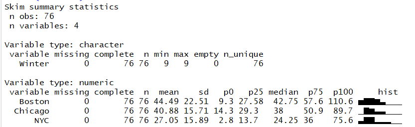
Figure 5.2: An example of skim() function output.
Next: some “interview questions”.